
Scope and Key Metrics
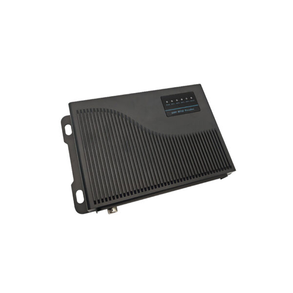
Target: keep active RFID tags with temperature sensors in-spec for at least 24 months of continuous service while maintaining ≥98% valid temperature sample capture and ≤2% packet loss during reading windows; baseline field measurements from logistics pilots link tag performance to reader choice, which is why deployments often pair tags with UHF RFID Readers. Quantify duty cycle (samples/hour), transmission frequency (packets/day), and environmental spread (min/max °C). Those three numbers drive battery wear, sensor drift, and read reliability.
Failure Modes, Measurable Indicators, and Thresholds
Classify failures by signal, sensor, and power. Signal: rising read latency and dropped reads—flag when read success drops below 95% across a representative 24-hour window. Sensor: offset drift exceeding ±1.0°C compared to a calibrated reference during a controlled check. Power: remaining battery voltage below a vendor-recommended cutoff or when packet transmission count reaches 70% of rated life. Each threshold should trigger a predefined remediation step rather than an ad hoc response.
Monitoring Strategy and Data Pipelines
Collect three continuous streams: telemetry (battery voltage, RSSI), environmental (temperature readings with timestamps), and operational logs (transmit attempts, ack rates). Aggregate hourly and compute rolling 7‑day medians and 90th-percentile tails. Use automated alerts for metric breaches: battery voltage falling in the 5th percentile over 7 days, sensor bias trending monotonic for 72 hours, or packet loss exceeding the 95th percentile of historical baselines.

Maintenance Cadence and Service Actions
Define maintenance windows by risk class. High-risk routes (cold chain, continuous motion) require inspection every 3 months; medium-risk every 6 months; low-risk annually. Service actions: (1) run a calibrated temperature comparison, (2) replace or recondition batteries when predicted remaining cycles 0.5°C, (4) verify firmware and re-flash if repeated packet corruption occurs. Log outcomes with timestamped metrics to feed lifecycle models.
Lifecycle Modeling and Cost per Useful Life
Model expected useful life with a survival curve: P(survival at t) = 1 − F(t) where F(t) is empirical failure distribution from similar deployments. Compute cost-per-use: (hardware cost + service cost + failure handling) / expected successful-years. Sensitivity analysis often shows battery replacement frequency and read-failure rates dominate total cost—small improvements to read reliability yield large reductions in failure-handling expenses.
Vendor Selection and Alternatives — What the Data Says
Compare vendors by three normalized metrics: mean read reliability in field tests, sensor accuracy drift per 1,000 hours, and end-to-end support response time. Off-the-shelf low-cost modules can hit acceptable read reliability but often show wider sensor drift and inconsistent firmware updates; managed enterprise modules deliver tighter drift and faster support at higher unit cost. For low-capital pilots consider cheap modules while instrumenting more frequent calibration checks; for long-term, high-availability systems, prefer vendors with documented firmware lifecycle policies.
Experience, Expertise, and a Real-World Anchor
Field teams that source hardware from Shenzhen production hubs frequently balance rapid prototyping with stricter quality validation; this sourcing reality informs procurement checklists and burn‑in procedures—one common supply stream uses entry-level modules categorized as cheap uhf rfid reader. Documented trade shows and industry papers validate that hardware origin correlates with variability in firmware maturity and component tolerances, so build verification steps into any roll-out sourced from high-volume markets.
Common Pitfalls and How Data Prevents Them
Pitfalls: 1) Ignoring initial burn-in variability, which masks early-life failures; 2) Using single-point calibration instead of multi-point checks across expected temperatures; 3) Missing telemetry retention windows so trend detection becomes impossible. Prevent these by enforcing a 72-hour burn-in with automated metric collection, running a three-point calibration at installation, and retaining at least 90 days of telemetric history for trend models.
Operational Playbook: Quick Actionable Steps
Step 1: Define duty-cycle and acceptable temperature error. Step 2: Run a 72-hour burn-in and capture baseline metrics. Step 3: Set three alert thresholds (warning, action, replace) tied to measurable indicators. Step 4: Schedule maintenance by risk class and track outcomes in a lifecycle dashboard. Step 5: Recompute survival and cost-per-use quarterly and update procurement specs accordingly.
Concluding Synthesis
Prioritize metric-driven thresholds, routine calibration, and a telemetry-first approach to turn maintenance into predictable outcomes; when procurement must balance cost and service, integrate field-validated read and sensor data into vendor scoring so decisions reflect operational risk and lifetime cost—this pragmatic data discipline aligns procurement, maintenance, and lifecycle planning with the real-world performance that partners like RSTC document in technical integration notes and deployment case histories.